How to lock cells in Microsoft Excel 2013
When you work in Excel with large tables, for example, price list, sometimes while scrolling you forget what columns you are watching. To make more comfortable work with tables you can fix position of cells (row or column) so that other cells to be scrolled and the cells with names are fixed.
In Microsoft Excel 2013 you can do it in 2 or 3 clicks, let’s see them
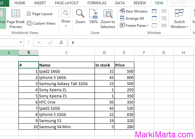
So you have a table in Excel (Drawing 1) with columns Number (#), Name, In stock and Price.
Figure 1. Excel table
And you want to fix column names so they are always on screen.
In ribbon you need to go to a tab "View" and find a button "Freeze panes".
Then select a row under that one you want to fix. In our case it’s a row with " 1 / Ipad2 / 16Gb /32 / 500". Press a button "Freeze panes" and in drop-down menu choose the first option "Freeze panes" and click it once (Figure 2).
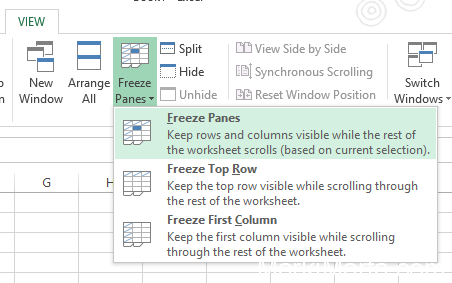
Figure 2. Freeze Panes
Now when you scroll a table, first row with column names is fixed.
If your table starts from the first row A1, then you can just go to "View", press "Freeze panes" and select the second item "Freeze Top Row".
 How to find the lines with the specific text in Linux console